A GPU Boids Simulator
The story behind the implementation of a GPU (OpenGL/OpenCL) particle simulator. Source code available here.
- Introduction
- The first steps
- First CPU boids draft
- Hello OpenCL
- Advanced mode unlocked
- Graphics update
- Perlin Target
- Final thoughts
Introduction
Creating a real-time physics-based simulation from scratch has been in the back of my mind since 2016. At that time, I was implementing a fluid-structure interaction solver to obtain my master degree in Computational Fluid Dynamics (CFD). Designed for industrial purpose, it was based on a super heavy finite element analysis framework. Imagine inverting sparse matrices with billions of variables at each frame… some of the 3D simulations took literally weeks of computations. When I discovered the rough but almost real-time approaches used for video games and 3D rendering (SPH, FLIP), I was astonished. I knew that one day I would find some time to develop a simulation of this kind.
Boids came in later. I have always been fascinated by murmurations, this swarm-like collective motion made of thousands of birds, all moving in an unexpected but total synchronisation. Then, a friend told me that a genius named Craig Reynolds had developed a “boids” model decades ago. It was simulating flocking behavior with 3 simple rules. I became more and more interested by his model, it sounded amazing to obtain, by simply using math and bits, these beautiful organic patterns. In addition, it was pretty simple to implement and looked like a very nice middle step before coding any fluid simulation. No need to deal with heavy Navier-Stokes equations (differential equations describing fluids motion), but it would still request the development of a point cloud renderer, a physics engine, a GUI window and a real-time application connecting them altogether.

Starling murmurations. Credit: Menno Schaefer / shutterstock
Besides, if boids simulations are quite common online, I noticed most of them are very limited in scale. There is actually a good reason behind it: the naive implementation of the boids model requests, for each particle, to loop over all the other ones. This is a very costly asymptotic complexity of O(N2), N being the number of particles. In other words, a small thousand of particles requires about a million of comparisons at each frame. For such heavy computations, it is hard to do anything consequent with CPUs and their limited number of threads. Fortunately, at the same time, I discovered the huge potential of GPUs and the field of GPGPU (General Programming GPU): basically using GPUs to do cool things beyond rendering a bunch of triangles.
This is how all the pieces fell into place in my head. Let’s do a boids simulator, it looks great and it will prepare the ground for a potential fluid simulation application. But let’s go big! Let’s do a full GPU particle simulation and display in real time millions of particles moving in a 3D world!
When starting this project one year ago, I was “a bit” optimistic. I really expected that, with OpenCL, simulating the movement of a million of particles would be a walk in the park. I was obviously wrong and if I stick to the previous metaphor, I ended up going in the mentioned park in the middle of the night with no light and a bunch of stray dogs hunting me. But it was fun and a very formative journey so I decided to write about it. This is the story of my experiments.
The first steps
The application
Creating an empty C++ desktop application from scratch can be a struggle. You need to connect all your dependencies: codebases, third-parties, environment scripts, build scripts… Everything must be at the right place with the right connection and the good options. Build it once, fail, fix it, build it twice, fail, fix it and try again. Concerning the build, if you want it to be a bit portable, you need to use CMake. You also definitely want to add a version control system, Git for example. Besides, it is better to add some formatting tools like clang-format to keep things clean and pretty. In addition, to have an application with its own cross-platform window, you need to use a specific third-party like SDL. If including OpenGL or OpenCL, you need to include specific APIs to connect to your GPU.
At that time, one of my friends introduced me to Conan and I happily embraced it. Conan is a wonderful C++ package manager which helps you including third-party libraries already built on remote servers by users or even automatically building them locally. Conan will generate a CMake file pointing to the different generated or retrieved binaries, making the third-parties integration significantly easier.
Overall, this is a lot of things to grasp and understand. It took me literally one weekend to figure this out, choosing the right third-parties, wandering through hollow error messages, stupid mistakes and finally making the whole thing consistent. All this installation step is definitely not straightforward and from my current perspective, after being done with all of that, I consider it as one of the hardest steps of the whole project. I think this is probably quite common among C++ developers to struggle with this initialization stage, because we usually work on big projects where someone else took care of setting up everything for us. How privileged we are.
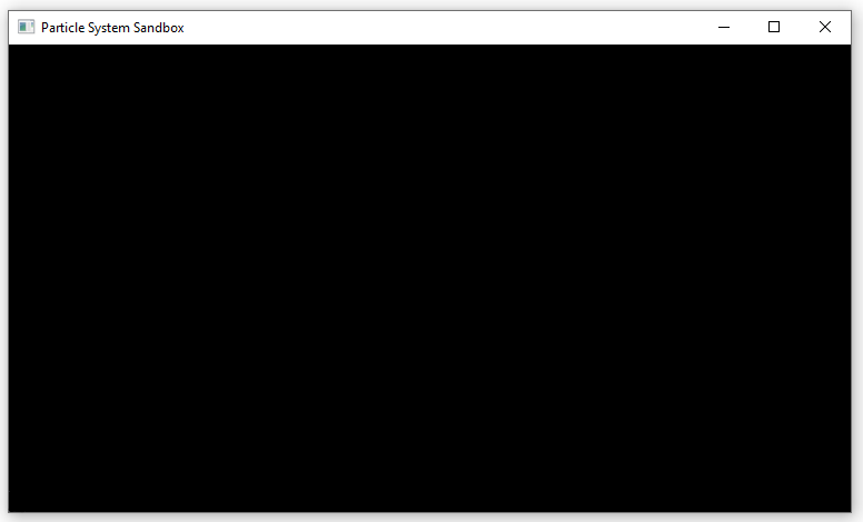
The great black window
The point cloud renderer
Okay, I have an empty window running on Windows. Great. Now I want to create a box in 3D and be able to move around. That’s another fun bit: implementing a 3D renderer. First of all, you need a GUI in which you will incorporate a 3D viewport. I choose Dear ImGui which is a light-weight, open source, friendly immediate-mode graphics user interface. See it as a fast way to prototype stuff, far away from more complete but heavy retained-mode Guis like Qt. At each frame, Dear ImGui will regenerate everything, there is no persistent storage of information. It is also directly incorporated in the rendering loop. All of this makes it easy to prototype and debug. Besides, it can be directly connected to SDL and OpenGL by using Glad, another third-party library in the mix!
With ImGui (let’s drop the Dear I am tired) in place, you can easily create some widgets, connect the mouse and the keyboards with SDL and have something interactive and responsive. Once this is done, the real work on the renderer begins with the implementation of shaders, camera, connection to mouse and keyboard. Using ImGui’s OpenGL context, drawing a box is pretty straightforward at that point. I add a bunch of points in it, with random positions and colors, those are my future particles on which I will apply the boids rules. After days of tweaking stuff, something is finally moving!
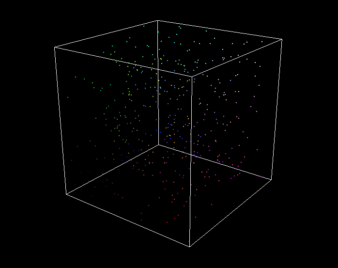
Box with particles
First CPU boids draft
The physics engine
Particles are finally here! Note that the renderer is only meant to display things and nothing else, it has no clue about boids or even physics. To make the particles behave like boids, we need a physics engine that will compute and update coordinates of each particle at every frame. In order to have a clean and clear codebase, I want stricly separated submodules, it helps a lot with debugging and potential futur development. Therefore, interactions between graphics and physics engines are limited as much as possible.
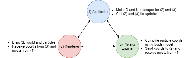
Triforce in action
Boids rules
Boids are considered as an emergent behavior, that is, a complex global behavior based on the interaction of a set of simple rules. Similarly to chaos behavior, it has no long term predictability but it differs from it by being predictable on the short term. This mix of chaotic and predictable movements makes this impression of a life-like phenomena. As presented by Craig Reynolds in 1986, its boids model is made of three rules :
- separation : steer to avoid crowding local flockmates
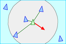 Credit: Craig Reynolds
- cohesion : steer to move towards the average position of local flockmates
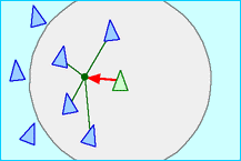 Credit: Craig Reynolds
- alignment : steer towards the average heading of local flockmates
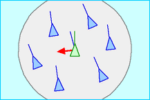 Credit: Craig Reynolds
As the weighted combination of these three rules can give a variety of different boids behaviors, their weights can be modified in the UI. On top of it, I also implement another optional rule to add an attractive/repulsive target, similar to a boids leader or a predator.
One physics engine iteration
At time t, the main application calls the physics engine and asks for an update of the particles coordinates. The engine applies boids rules with coordinates and velocity of each particle at t-1 to compute acceleration at t. It then integrates these accelerations by dt (time spent between t-1 and t) to obtain velocities and finally coordinates at t. During the process, various normalizations and clampings occurs on velocity and coordinates, depending on the selected boundary conditions and maximum speed. Once the computation is done, we still need to load these new coordinates on the GPU to render them, remember, this first draft is CPU-based. Hence, we need to transfer coordinates buffer from CPU to GPU at each frame. This step can be costly for big number of particles.
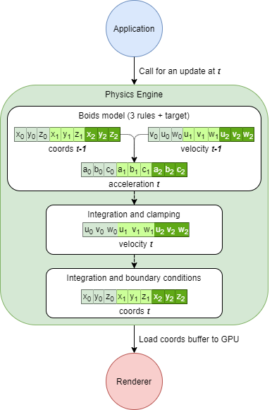 Physics Engine at work
For this first CPU implementation, I have the chance to be assisted by a very good friend of mine who is experimented in numerical arts and wants to get a hand on software development. After a bit of tweaking and debugging, we start seeing organic patterns and finally the expected boids behavior. I take some time to optimize the data flow but we quickly reach performance limitations with only 103 particles. This is 2-3 orders of magnitude below my ultimate goal, it is time to bring in the GPU artillery!
 CPU - 1k - 60FPS
Hello OpenCL
OpenCL framework
OpenCL is the Khrono’s open framework for heterogeneous programming, giving access to GPUs among other things. It supports task-parallelism, data-parallelism and explicit vectorization accross a various range of platforms. We can compare it to Nvidia CUDA solution when using GPUs. In an OpenCL application, workload is shared between host and devices:
Host : usually a CPU running the main program, it manages the device and prepares the ground for the computation. On the selected device, it implements kernels (shaders) definitions, memory buffers, kernels parameters values and so on. It also decides host-device memory transfers.
Devices : they do the heavy lifting of the processing in a massive parallel fashion using thousands of threads and explicit vector processing. We use a single GPU as an OpenCL device in our case.
That is a lot of added complexity compared to the original CPU solution and playing with GPUs is challenging, but used carefully OpenCL can bring huge performance improvements.
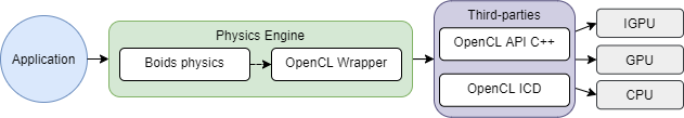
To have access to GPU power through OpenCL, we need to add some extra steps to our processing. First, we use Conan to retrieve the OpenCL C++ API. We also need the OpenCL ICD (installable client loader), usually available in device vendors dev kits (CUDA, Intel SDK). The ICD is a dll allowing us to select an available OpenCL device, build its device-specific binaries and run the kernels on it. Now, to keep everything clean and simple, we need to add an extra OpenCL layer in the physics engine because we don’t want to have direct OpenCL calls in our boids submodule. Physics is one thing, host-device communication another. Besides, OpenCL calls are generic and will probably be used by other physics submodules at some point. Hence, the arrival of an OpenCL wrapper, doing the interface between my physics engine and the OpenCL API.
 Connecting to OpenCL devices
Interop OpenGL/OpenCL
Apart from increasing performance by massively using data-parallelism, OpenCL also removes costly CPU-GPU transfers. With CPU boids implementation, we had to transfer all new coordinates to GPU renderer at every frame, remember? When you have a few hundreds of entities, no big deal, but when you start playing with hundreds of thousands of them, it means transferring a few mega octets between GPU and CPU at every frame. It can strongly impact performance.
Fortunately, interoperation is supported between OpenGL and OpenCL. Basically, OpenGL and OpenCL can share specified GPU memory buffers and therefore ensure zero copy between computing and rendering steps. When starting its processing, the physics engine takes full control of the coordinates buffers and passes it back to the renderer when done. Beautiful isn’t it? It requires some adjustments, though. You need to ensure that OpenCL is using OpenGL context and that both frameworks are using the same device, that means I need to add some logic in the OpenCL wrapper to detect which device (IGPU or dedicated GPU) is used to render the application and use it for the physics processing. So, make sure that you launch the application with your most powerful GPU as it will be used for both rendering and processing.
After loosing some evenings and nights in debugging mode, it finally behaves the same way as with CPU, nice. Obviously, my next febrile move is to increase as much as I can the number of particles. After a bit of adjustements at kernel level, I finally cap at 30k particles for 60 FPS. Wait, what? 30k? Where is my million?
 GPU - 30k - 60FPS
Advanced mode unlocked
Space Partitioning
OpenCL does increase performance by more than an order of magnitude, from 1k to 30k, but this is not enough. To go further, it is time to focus on a well known problem in the N-body simulation world, the nearest neighbor search bottleneck. For this type of simulation, NNS algorithms are critical. You have N particles and each particle is under the influence of its neighbors from a given vicinity, you need to compute this effect but how do you find those neighbors among N? Brute force algorithm loops over all N particles to check the distance between the two particles, the one considered and its potential neighbor, giving us an asymptotic complexity of O(N2). Using thousands of GPU threads doesn’t fix the problem as every thread will still have to run this potential huge loop, hence the previous performance cap at 30k. Luckily, there is a vast litterature on the NNS subject with smarter solutions. After reading a small dozen of articles, I decide to go for Simon Green’s simple but very efficient proposition based on a combination of spatial partitioning and sorting.
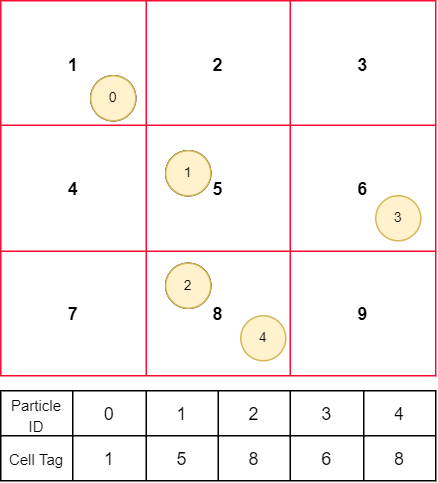
The idea is to split the 3D world in small cubic cells and tag each particle with the cell ID where it is found.Once every particle has been tagged, it is then possible to focus the search only in the neighboring cells. Implementing this spatial partitioning step is quite straightforward with a box for 3D world. You have a direct connection between particle position and cell index that can be used as an unique ID.
 Spatial Partitioning
In order to debug it, the cell grid is sent to the renderer and displayed with the particles. Pretty neat visual effect in bonus!
 3D Grid cell
Radix Sort
To get rid of the O(N2) constraint without complex mapping between cells and particles, we need to sort the particle buffers by using their cell ID tag. Doing so allows us to loop among very small and specific subsets of the global buffers (coordinates and velocity) while computing the boids rules.
Compared to the spatial partitioning, the sorting step is trickier. Good news is efficient parallel sorting algorithms, radix sort and bitonic sort, can be found online. Both seem to be super fast. After some testing, I decide to go with radix sort as there is one very nice open-source OpenCL implementation on github and it seems slightly faster than bitonic sort. A dozen evenings of hard work are necessary to adapt and plug the algorithm correctly to my OpenCL wrapper and boids model. Implementing this GPU spatial partitioning + radix sort + boids model pipeline is probably the hardest part of the whole project, a lot of pain fun involved. Many things can go (and will) go wrong at the different steps of the process and I need to debug it based on some emergent behavior hardly predictable.
For the record, I even got stuck with a terrible bug for weeks without noticing it, naively assuming that with a lot of particles involved, things can be a bit messy. It is only after unloading global buffers at each step for something else that I realized that everything was broken because a refresh was missing in the radix sort at the beginning of each frame.
Notice the particles crossing each other? That’s a bug.
The new physics engine iteration
We now have a more complex pipeline in the physics engine. At each time frame, we start by tagging all particles with their cell IDs and store this information in a new global cell tag buffer. Once done, we can sort it and use it to permutate other global buffers (coordinates, velocity and acceleration). Still with the global cell tag buffer, we can also scan it in order to know how many particles are in each cell and generate the grid start/end particle indices buffer. This new buffer provides for each cell the first and last particle indices in global buffers. This is very important for the boids model, as it allows us to apply the boids rules on every particle without looping on the whole global buffers for the NNS phase. Using this buffer, we can now analyze very specific and limited parts of the global buffers where we are certain to find potential neighbors.
Once done, the rest is similar to the previously explained CPU prototype. Note that absolutely everything detailed above is done on GPU. There is no CPU-GPU memory transfer at computing or rendering steps, except when sending the kernel and shader parameters.
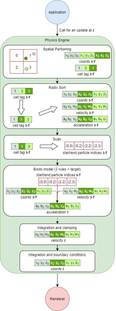 Advanced GPU physics engine pipeline
Optimization and limitations
At that point, I can focus on kernels optimization, the theorical O(N2) barrier is gone so there is room to make things faster. I improve the critical boids kernels bit by bit, streamlining the process, improving the data flow, removing unecessary steps, tweaking the parameters.
The main drawback of the spatial partitioning is that it can still contain hidden asymptotic complexity of O(N2). Indeed, if every particles are in the same cell, you are back to square one, looping on every one of them for the NNS step. With the right cell resolution, this can be prevented in most cases, but in not all of them. The O(N2)-induced lagg appears when an attractive target is added to the system and all particles converge to it, in these cases the drop of FPS is sharp. One easy solution is to limit the number of particles visited in each cell at the NNS step: “visit the 15 000 first neighbors in this cell and forget the remaining ones”. This is not perfect as it can generate noticable visual artifacts in boids behavior and it is not a pure boids model anymore.
I also go deep into the algorithms, trying to implement GPU local memory use in the kernels. I won’t go too much into details for this one as it would mean explaining the complete memory framework of OpenCL, but in short it don’t work well for this type of application. At first, I am a bit surprised by the results because usually using local memory over global memory means significant performance improvements. However after looking at different other GPU N-body simulation implementations, it appears that my lack of success with local memory is quite common for this type of simulation. The performance with global memory is higher thanks to a hidden phenomenon due to the sorting of the particles, it is called coalesced memory access. Basically the memory transactions are drastically improved in this case because neighboring threads work on neighboring sorted particles and use the same data for the computation, reducing costly memory transaction with global memory.
After weeks of work, I finally reach the stage of 260k particles running in real time at around 60 FPS with my Nvidia GTX1060. Jumping from 1k to 260k, not bad. I can definitely go higher, things are far from being perfect but I am very happy with the results and it is already a lot of particles, the box has been expanded 3 times already and is still overwhelmed by boids. The 1 million particles objective can wait, I will be more humble next time.
GPU - 260k (spatial partitioning + radix sort) - 60FPS
Graphics update
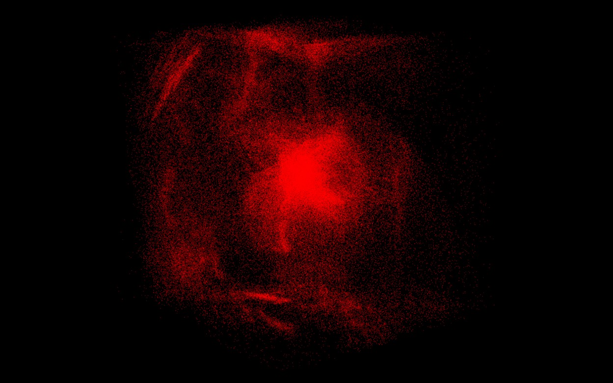
So here I am, a smile on my face, a few hours of sleep lost and 260k particles running smoothly on my machine. One thing which is still bugging me, though, is the visual aspect of the simulation. I haven’t spent much time working on it as the original plan was to work on GPGPU performance and advanced computation. Nevertheless, it is time for a small graphics enhancement to make things agreable to watch, right now it is pretty ugly to be honest. Fortunately, I am pleasantly surprised by the numbers of hardcoded features available in the old OpenGL state machine. In a few lines, I am able to add some antialiasing, point smoothing and additive blending, I also put some colors in the mix. Contrasts are striking.
I also slightly refine the vertex shaders to have a point size changing in function of the distance with the camera. It gives an impression of depth. Doing so, I notice that sometimes some particles in the background are drawn on top of front ones, not good. To prevent it, I need to compute the particle-camera distance for every particle and sort all the global buffers again in function of this distance. Performance are not even impacted by the second sorting, proving how fast the radix sort is!
Distance-dependent particle size
Additive blending
Perlin Target
One last thing, I want to implement a moving target in the 3D world. The current one is static in the center of the box. First, I think about letting the user control it but he can already control the camera rotation and translation with mouse and keyboard, usability will get tricky. Thus, I prefer to implement a random automatic trajectory and let the user admire it.
Perlin noise is the perfect solution for this problem. Invented by Ken Perlin in 1983, it gives a more lifelike, natural randomness than classical random value generators. Based on a 3D grid with pseudo random gradient values set at its vertices, it generates random values in 3D space with some spatial coherency. My implementation is based on an open-source C++ version of the algorithm. By arranging a unique Perlin noise generator with different gradients for each spherical coordinates, I am able to implement a target moving smoothly in the box around its center. This results in an impression of flocks chasing after some food for the attractive behavior or fleeing a predator for the repulsive behavior.
Target with Perlin trajectory
Final thoughts
Well, I think it is time for a conclusion, this post is long enough!
All in all, it was an amazing experience. I remember very well the first weekend I spent on this project, almost one year ago, when I was struggling with an empty black window. I am quite amazed by how far I managed to go with some skills and a good amount of dedication. I have definitely learned a ton about GPGPU, software development but also about myself. Working alone in the evening after spending the day on your daily developer tasks takes some determination. Nobody will go after you if the project is not moving, you are on your own and running away from your screen is tempting.
Of course there is still a lot of things to improve or implement (more optimization, more advanced boids model, bug fixes…), but there will always be. I think it is time to move on to something else. So what’s next? Well, good question, maybe a visualizer comparing different parallel sorting algorithms or a Vulkan renderer from scratch. Of course I haven’t forgotten about the fluid simulation either! We will see how it goes.
If you want to play with the boids or have a look at the code, everything is available here. Have fun!
If you read this line, it means you have been patient enough to go through all my gibberish, thanks a lot for your interest and don’t hesitate to contact me if you have any question!