Position Based Fluids

12 Oct 2021 in RealTimeParticles

Implementation of a real-time Position Based Fluids simulator. Source code available here.

1. Introduction
2. Simulating Fluids with Math and bits
   1. Eulerian or Lagrangian. To be or not to be?
   2. Lagrangian computational methods
      1. The old venerable master
      2. A newcomer in town
   3. Position Based Fluids equations
      1. Introduction to constraints
      2. Simulation loop
3. Implementing a Position Based Fluids model
   1. From the first integration steps…
      1. Switching between physical models
      2. Implementing the fluid kernels
   2. … to a functioning real-time fluid simulation
      1. Give me back my fluid particles Varus!
      2. Adjusting time and space to fluid imperatives
      3. Focus on initial and boundary conditions
      4. Advanced features
4. Conclusion

Introduction

To acquire knowledge and expertise in a domain, I tend to mostly rely on two mechanisms:

1. Aim high (sometimes stupidly high)
2. Split complex challenges into smaller ones to tackle them separately

Following and combining those two basic principles usually works pretty well for me. I set myself high goals far ahead, divide the path to them into a multitude of intermediary steps, and patiently reach everyone of them to finally arrive at the ultimate objective.

Therefore, the boids behaviour model described in my latest post was just a step. I greatly enjoyed it but it was above all an intermediary and necessary stage. I had something more complicated in mind, a physical model like fluids or combustion, but I wanted to separate theoretical and technical challenges.

Boids project was all about setting up a C++ project from scratch, creating an OpenGL render, an OpenCL wrapper and connecting them altogether. No significant theoretical obstacles but a lot of technical difficulties to be managed one by one. Real physical models usually come with complex ordinary or partial differential equations (ODE/PDE), adding another mathematical layer of complications. I wanted to have a solid foundation before diving into it.

Well guess what, boids simulation being fully functional, now is the time for the real game. Let’s implement a real-time 3D fluid simulation!

Simulating Fluids with Math and bits

I always found amazing that something as complicated as fluid dynamics can be modelized by a few differential equations. Fluid motions can be incredibly complex, both temporally and spatially, nevertheless some 19^th century geniuses, namely Claude-Louis Navier and George Gabriel Stokes, introduced a pair of PDEs and showed that by approximately solving them you could get very close from many fluid behaviors present in our world. Crazy, right? I say approximately because the Navier-Stokes equations have no analytical solutions in 3D and are therefore solved using numerical or analytical models based on different approximations. So before implementing anything, we need to decide which of these approaches best suits our needs.

By the way, if you have 3D solutions of Navier-Stokes equations written on your fridge, don’t hesitate to share them to the world as they are among the seven most wanted open problems in mathematics ($1 million prize). \[\begin{aligned} \nabla \cdot \mathbf{u} &= 0 \\ \rho ( \frac{\partial \mathbf{u}}{\partial t} + \mathbf{u} \cdot \nabla \mathbf{u} ) &= - \nabla p + \rho \mathbf{g} + \mu \nabla^2 \mathbf{u} \end{aligned}\]

Miss Equation 1822, the Navier-Stokes equations (Eulerian description for a viscous incompressible fluid)

Eulerian or Lagrangian. To be or not to be?

Before delving into numerical schemes and solvers, first we need to choose between two different ways of looking at fluid motion:

1. Eulerian description - We look at the fluid domain globally, considering it as a vector field. The fluid behavior is analyzed and solved over time at specific fixed places in the studied domain. This concept is widely used in the field of Computer Fluid Dynamics (CFD) where scientists and engineers apply it to analyze and solve real world fluid problems, for example reducing aircraft drag or improving the efficiency of wind turbines. This approach can give very accurate estimates of flow motions and forces. I used it in my master thesis as most of the people of my Fluid Lab. Unfortunately it can be extremely costly, some 3D heavy simulations literally take weeks or months to proceed. Besides, particles movements can only be obtained by post-processing the fluid velocity field as they are not directly taken into account in the solver.

2. Lagrangian description - We consider the fluid as a group of individual particles, analyzing their interactions to determine their trajectories and conditions. Unlike the Eulerian approach, the domain is not considered as a whole and its importance is less significant. No need of mesh or grid, simply a bunch of particles on which we apply some rules modeling fluid interactions. To make it simple, it is a bit like approximating a fluid domain with a ball pit. Historically, Lagrangian simulations have been considered less precise than Eulerian ones. One of their biggest forces is their execution speed, they can be used for coarse but fast simulations giving visually acceptable results. Thus, they are particularly appreciated in the world of Computer Graphics. By being meshfree, it is also well suited for free-surface problems or ones with large boundary displacements.

In short, using Lagrangian description can help us favoring interactivity over accuracy. Hence, a Lagrangian solver clearly seems to be the right candidate for our real-time particle simulator. We “simply” need to apply the right combination of rules on each particles to give them a sense of fluid motion. This is the subject of the next part.

Lagrangian computational methods

The old venerable master

Smooth Particles Hydrodynamics (SPH) is one of the major computational methods used in Computer Graphics for fluids. Initially developped by Gingold, Monaghan and Lucy in 1977 for astronomical problems (article), since then it has been widely used in fluid simulations, for its simplicity of implementation and execution. Combined with post-processing rendering, it can provide very realist free-surface simulations.

SPH method divides the fluid continuum in a set of discrete particles. For each particle, SPH interpolates its fluid properties using functions to weight the influence of its neighbouring particles. Called smoothing kernel functions, those functions are a central part of the method. They determine how particles interact with each other and must be carefully designed. Using this method, we can compute pressure and viscosity forces on each particle and deduce its acceleration using Newton’s second law. Particle velocity and position are then obtained by integration. To facilitate nearest neighbor search (NNS), SPH method can also use some spatial partioning. Particles, sum of neighbors contributions, spatial partitioning… sounds familiar, doesn’t it? Don’t be surprised, it is strongly similar to my boids implementation and that is very good news.

\begin{equation} A(\mathbf{x}) = \sum_j m_j \frac{A_j}{\rho_j} W(\mathbf{x} - \mathbf{x_j}, h)\end{equation}

Interpolation at \(\mathbf{x}\) of a scalar quantity A by a weighted sum of contributions from its neighbor particles \(j\) \[\begin{aligned} W_{poly6}(\mathbf{r}, h) = \frac{315}{64 \pi h^9} & \left\{ \begin{array}{lr} (h^2 -\Vert r \Vert^2)^3 & 0 \leq r \leq h\\ 0 & otherwise \end{array} \right. \\ W_{spiky}(\mathbf{r}, h) = \frac{15}{\pi h^6} & \left\{ \begin{array}{lr} (h - \Vert r \Vert)^3 & 0 \leq r \leq h\\ 0 & otherwise \end{array} \right. \end{aligned}\]

Exemple of smoothing kernel functions used in our model and mentioned in Muller et al., 2001

Despite its charms, after reading a few papers on SPH, I realized that it might not be the perfect solution. Traditional SPH model can quickly show instabilities when some particles have few or no neighbors, injecting negative pressure in the domain. There is a vast number of variants made in the last decades to address those issues and improve the initial model, PCISPH, XSPH… Modern SPH results are much better, but the use of small time steps for the simulation is still necessary, limiting simulation speed. Hence, even if you manage to have a simulation running at 60 fps, the motion of particles might still be visually very slow.

A newcomer in town

While reading a well-known fluid SPH paper called Particle-Based Fluid Simulation for Interactive Applications written in 2001, one name caught my attention: Matthias Muller. He is currently the physics research lead at NVIDIA and I remembered seeing another computational method on his personal blog a while ago.

Called Position Based Dynamics (PBD), this framework was presented in 2006 and has been used for fluid simulation in a paper named Position Based Fluids (PBF). It was published in 2013 by Muller and Macklin, 12 years after the initial SPH paper. Personal rule of thumb; when scientists wrote a paper on the same subject 10 years after the previous one, it is usually a good idea to read it, they probably have something better to propose. Indeed, this PBF paper brought great insights to this new method but also highlighted the limitations of the SPH model. It also helped me understand the differenciation between two key notions used in this field: interactive vs real-time. The first one means fast enough to play with interactively but potentially still visually too slow to be acceptable in many applications, the latter means interactive and fast enough for video games type application, exactly what I am looking for.

Many computation methods, SPH included, are based on Newton’s second law. Compute the forces applied on each particle, use it to obtain its acceleration and from there integrate it twice to get its position. Repeat it for each time step and you now have motion. Position Based Dynamics/Fluids approach is radically different, you don’t even compute the acceleration, you mostly focus on particles positions and constraints.

Constraints are designed functions defining wanted system behavior, how you want the particles to be positioned regarding each other. You can imagine one constraint as a web connecting one particle to its neighbors and constraining them in order to have some physical property (energy, density or else) enforced at its desired value. I find this approach very interesting. No double time integration and more explicit control on your system, as you manipulate directly particle positions. To improve precision and get closer to the wanted behavior, you can iterate on your constraint system at each time step. By doing so, PBD offers more stability and allows us to increase simulation time steps, bringing us into the real-time world.

Position Based Fluids equations

Introduction to constraints

In their article, Macklin and Muller give a good overall presentation of their proposed framework. It is quite consequent and contains different specific ramifications and fine-tuning so I won’t go into every details. Instead, I want to focus on the key concept of constraint because it took me a while to understand it completely and I think its comprehension is crucial for any PBF implementation.

For each particle \(p_i\), Position Based Fluids approach sets a single positional constraint \(C_i\) on \(p_i\) itself and its neighbors, all their positions being contained in \(\mathbf{X} = [\mathbf{x}_1, \ldots, \mathbf{x}_n]\) with \(i \in [1, \ldots, n]\). The objective is to constrain each particle to reach a position \(\mathbf{x}_i\) where its density \(\rho_i\) tends towards the rest density \(\rho_0\), a fluid-dependent property defined by the user. \[C_i(\mathbf{X}) = \frac{\rho_i}{\rho_0} - 1 \tag{1}\]

Interestingly, we rely on a SPH kernel function \(W\) to compute \(\rho_i\). In their article, they use the smoothing kernels \(W_{poly6}\) and \(W_{spiky}\) introduced previously. \[\rho_i = \sum_{j = 1}^n W_{poly6}(\mathbf{x}_i - \mathbf{x}_j, r) \tag{2}\]

For every constraint, we want to find the set of positions \(\mathbf{X}\) which forces the density \(\rho_i\) to be equal to \(\rho_0\). Mathematically, it means that we want to find the particles positions correction \(\Delta \mathbf{X}^i = [\Delta\mathbf{x}_1^i, \ldots, \Delta\mathbf{x}_n^i]\) giving us: \[C_i(\mathbf{X} + \Delta \mathbf{X}^i) = 0 \tag{3}\]

From there, we can try to minimize the constraint \(C_i\) by iterations with a gradient descent. To do so, we linearly approximate \((3)\) and assume that \(\Delta \mathbf{X}^i\) is in the direction of the negative gradient of \(C_i\). Considering \(\nabla C_i = \nabla_{\mathbf{X}} C_i = [\nabla_{\mathbf{x}_1} C_i, \ldots, \nabla_{\mathbf{x}_n} C_i]\) : \[\Delta \mathbf{X}^i \approx \nabla C_i(\mathbf{X}) \lambda_i \tag{4}\] \[\begin{aligned} C_i(\mathbf{X} + \Delta\mathbf{X}^i) & \approx C_i(\mathbf{X}) + \nabla C_i(\mathbf{X})^T \Delta\mathbf{X}^i = 0 \\ & \approx C_i(\mathbf{X}) + \nabla C_i(\mathbf{X})^T \nabla C_i(\mathbf{X}) \lambda_i = 0 \end{aligned} \tag{5}\]

At this point, we can deduce the value of the density constraint coefficient \(\lambda_i\) : \[\lambda_i = - \frac{C_i(\mathbf{X})}{\sum_{j = 1}^n {\mid \nabla_{\mathbf{x}_j} C_i(\mathbf{X}) \mid}^2 } \tag{6}\]

Besides, using the SPH discrete definition of the density \((2)\), we can define more precisely the gradients of \(C_i\) with respect to each particle: \[\nabla_{\mathbf{x}_k} C_i(\mathbf{X}) = \frac{1}{\rho_0} \left\{ \begin{aligned} & \sum_{j = 1}^n \nabla_{\mathbf{x}_i} W_{spiky}(\mathbf{x}_i - \mathbf{x}_j, r), \space k = i \\ & - \nabla_{\mathbf{x}_j} W_{spiky}(\mathbf{x}_i - \mathbf{x}_j, r), \space k = j \end{aligned} \right. \tag{7}\]

Remember that for each particle we set one constraint affecting this particle but also its neighbors. Hence for each particle, its position is corrected by its own constraint but also the ones set on its neighborhood. Macklin and Muller superpose each contribution: \[\Delta \mathbf{x}_i = \sum_{j = 1}^n \Delta \mathbf{x}^j_i = \sum_{j = 1}^n \lambda_j \nabla_{\mathbf{x}_i} C_j(\mathbf{X}) \tag{8}\]

Finally, by connecting \((7)\) and \((8)\) and assuming \(\nabla_{\mathbf{x}_i} W_{spiky}(\mathbf{x}_i - \mathbf{x}_j, r) = -\nabla_{\mathbf{x}_j} W_{spiky}(\mathbf{x}_i - \mathbf{x}_j, r)\) (\(W_{spiky}\) being symmetric), we obtain: \[\Delta \mathbf{x}_i = \frac{1}{\rho_0} \sum_{j = 1}^n (\lambda_i + \lambda_j)\nabla_{\mathbf{x}_i} W(\mathbf{x}_i - \mathbf{x}_j) \tag{9}\]

That’s it, our constraint system is set up. For each particle, we set a constraint, compute its density, deduce its lambda and obtain the position correction from there. At each time step, we will repeat this process several times to get closer from the rest density everywhere in our system.

Simulation loop

Now that the position correction algorithm has been explicited, we can have a global overview of the simulation loop called at each time step.

 

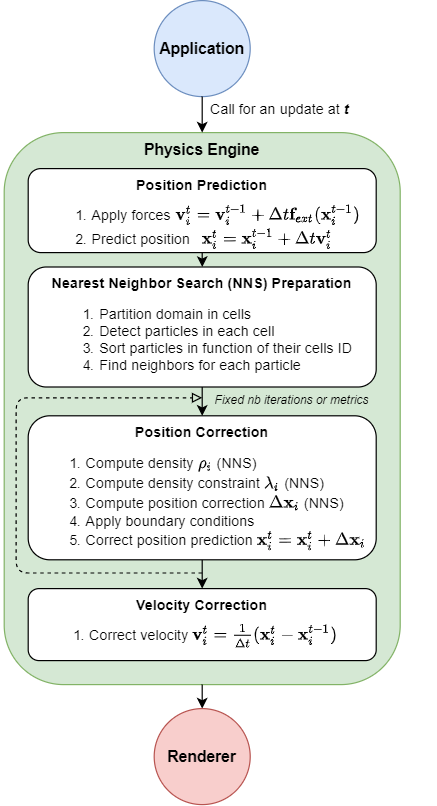Position Based Fluids simulation loop

 

1. Position Prediction - First we update the velocity of each particle by integrating its acceleration due to external forces. Using this updated value, we predict the next position of the particle. This prediction will be corrected later in (3) to enforce density constraints.
2. Nearest Neighbor Search Preparation - To avoid O(N²) time complexity (N being the number of particles), we spatially partition the domain and sort the particles by their cell ID. I already explained this process in the boids implementation post so I won’t go into details. Just note the fact that we do this processing only once for each time step, this is a performance-accuracy trade-off working well up to a certain time step range.
3. Position Correction - Central piece of the Position Based Fluids algorithm, it is based on the constraint concept explained in the previous section. We correct the position in several iterations at each time step. To decide when to stop the correction, we can use some qualitative metrics or simply set a fixed number of iterations. In their article, Muller and Mackling iterate a constant number of times in order to keep the framerate steady.
4. Velocity Correction - Once the position has been corrected, we recalculate the velocity based on this new value. Note that the algorithm requires to maintain two separate position buffers, one at t-1 and another one at t. We usually swap the two buffers at this stage to prepare the next time step iteration.

This is a quick overview which does not include all the specific pieces implemented for more realistic visuals. In their paper, Muller and Macklin add a constraint force mixing (CFM) term while computing the density constraint to avoid division by zero. They add an artificial pressure term to prevent particle clustering due to a lack of neighbors. This repulsive term generates a surface tension effect which results in very interesting visuals. They also introduce some vorticity confinement in the last part of the simulation loop to counter the energy loss generated by the PBF framework. Finally, they apply XSPH viscosity, a concept coming directly from the SPH literature which produces a more coherent motion. Yes, it all sounds like a cooking recipe. I quickly realized that fluid simulations in computer graphics are less rigorous than in CFD field. As long as it brings something visually, you can insert some non-physical components in the equations.

Implementing a Position Based Fluids model

From the first integration steps…

Switching between physical models

Since the beginning of the RealTimeParticles application, I have planned to implement different physical models and to switch between them through the UI. So, even before working on it, the ground work for the PBF integration is already halfway. Thanks to classic polymorphism, secure encapsulation and different existing subsystems APIs, it is quite trivial to add a new physical model from scratch. The tricky part comes from the OpenCL wrapper being a singleton. I need to be able to switch between different models using potentially similar buffers or kernels on the OpenCL device. For example, both boids and fluid models use the spatial partioning framework and its radix sort. I don’t even want to think about the nightmare that could arise from this unwanted cohabitation on the OpenCL device side. The singleton should be preserved but I have to clean the kernels and the buffers every time I change my physical model. This is also a good opportunity to do a clean separation between the different kernels by storing them in separated .cl files. The OpenCL context will now call a specific subset of those files for each model.

// file: "Fluids.cpp"
CL::Context& clContext = CL::Context::Get();

std::ostringstream clBuildOptions;
clBuildOptions << "-DEFFECT_RADIUS=" << Utils::FloatToStr(1.0f);

clContext.createProgram(PROGRAM_FLUIDS, { "fluids.cl", "grid.cl", "utils.cl"}, clBuildOptions.str());

A cleaner way to initiate models on OpenCL side

Implementing the fluid kernels

Let’s put into practice the principle of splitting everything into small steps. I will start with a simplistic model only including gravity, without constraint or correction of position. I simply assemble a skeleton with the position prediction step, the NNS and the velocity update. Unsurprisingly, it essentially gives me rain-like motion. Maybe I could just stop here, isn’t it a fluid simulation after all? Hum, nevermind… time to dive into the kernels.

 

Rain Simulator 2021, only for 2.99$

The real work can begin, we have to implement the kernels used in the correction loop. After a quick review, I count four kernels to generate; one to compute the density, one for the density constraint \(\lambda\), another one for the position correction and a final one to correct the position. As mentioned in the graph above, the first three operations need a neighbor search so we might run neighbors searches a small dozen times for each time step. This will be significantly costly in terms of performance. In comparison, for the boids we only performed this operation a single time at each time iteration. Besides, note that this is only for the basic implementation, without any artificial pressure or vorticity confinement tricks.

But before analyzing performance, we need the bricks that will be used in all these kernels: the smoothing kernel functions \(W_{poly6}\) and \(W_{spiky}\). The latter one is only called under its gradient formulation, so no need to implement it directly. Here are the proposed implementations:

// file: "fluids.cl"
/*
  Poly6 kernel mentioned in
  Muller et al. 2003. "Particle-based fluid simulation for interactive applications"
  Return null value if vec length is superior to effectRadius
*/
inline float poly6(const float4 vec, const float effectRadius)
{
  float vecLength = fast_length(vec);
  return (1.0f - step(effectRadius, vecLength)) * POLY6_COEFF * pow((effectRadius * effectRadius - vecLength * vecLength), 3);
}

/*
  Gradient (on vec coords) of Spiky kernel mentioned in
  Muller et al. 2003. "Particle-based fluid simulation for interactive applications"
  Return null vector if vec length is superior to effectRadius or inferior to FLOAT_EPS
*/
inline float4 gradSpiky(const float4 vec, const float effectRadius)
{
  const float vecLength = fast_length(vec);

  if(isless(vecLength, FLOAT_EPS))
    return (float4)(0.0f);

  return vec * (1.0f - step(effectRadius, vecLength)) * SPIKY_COEFF * -3 * pow((effectRadius - vecLength), 2) / vecLength;
}

\(W_{poly6}\) and \(\nabla W_{spiky}\) implementations

For the rest, each kernel is relatively similar, we start by doing a NNS to retrieve the neighbors and then compute each neighbor contribution.

// file: "fluids.cl"
/*
  Compute fluid density based on SPH model
  using predicted position and Poly6 kernel
*/
__kernel void computeDensity(//Input
                              const __global float4 *predPos,      // 0
                              const __global uint2  *startEndCell, // 1
                              //Param
                              const     FluidParams fluid,         // 2
                              //Output
                                    __global float  *density)      // 3
{
  const float4 pos = predPos[ID];
  const uint3 cellIndex3D = getCell3DIndexFromPos(pos);

  float fluidDensity = 0.0f;

  uint cellNIndex1D = 0;
  int3 cellNIndex3D = (int3)(0);
  uint2 startEndN = (uint2)(0, 0);

  // 27 cells to visit, current one + 3D neighbors
  for (int iX = -1; iX <= 1; ++iX)
  {
    for (int iY = -1; iY <= 1; ++iY)
    {
      for (int iZ = -1; iZ <= 1; ++iZ)
      {
        cellNIndex3D = convert_int3(cellIndex3D) + (int3)(iX, iY, iZ);

        // Removing out of range cells
        if(any(cellNIndex3D < (int3)(0)) || any(cellNIndex3D >= (int3)(GRID_RES)))
          continue;

        cellNIndex1D = (cellNIndex3D.x * GRID_RES + cellNIndex3D.y) * GRID_RES + cellNIndex3D.z;

        startEndN = startEndCell[cellNIndex1D];

        for (uint e = startEndN.x; e <= startEndN.y; ++e)
        {
          fluidDensity += poly6(pos - predPos[e], fluid.effectRadius);
        }
      }
    }
  }

  density[ID] = fluidDensity;
}

Density kernel

The density constraint and correction kernels are slightly harder to implement as the maths behind are a bit more involved but it is still doable. The trickiest part is how \(\nabla_{x_k} C_i\) definition changes depending on whether \(k = i\) or not. Despite those small complications, I finally get to the point where the whole simulation loop is ready to roll. Before runnint it, I fix a multitude of glitches in the different kernels, double check every implementation by comparing it to the theory. Alright, everything seems coherent, let’s see how it looks like (drumroll please)…

 

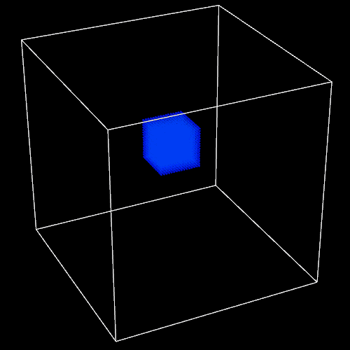
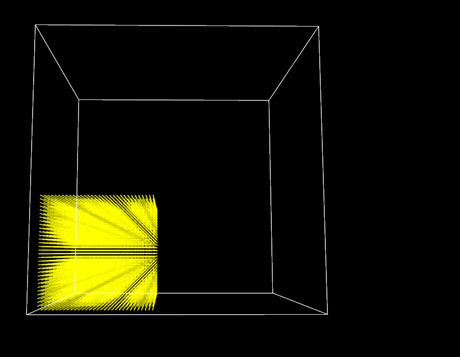
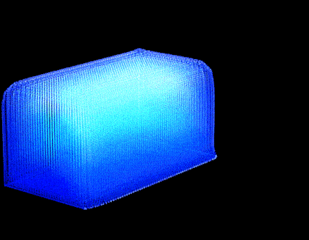
Very first capture of my “fluid” simulation, nice try

… to a functioning real-time fluid simulation

In the next section, I intentionally take a dramatic tone to highlight the tough but necessary debugging phase that so many developers encounter but don’t always talk about. Don’t worry, no keyboards were harmed in the making of this project.

Give me back my fluid particles Varus!

So this is where the fun begins. Theory, checked. Basic implementation, checked. Yet, nothing is working as expected. In the scene shown above, you can discern some Rorschach patterns but no fluid in sight. There are so many potential failure factors here that it is a bit frightening. Maybe I misunderstood the theory, maybe there is a bug in a secondary kernel or even a data race on GPU side. I might use wrong parameters values or buggy initial conditions. Maybe everything is working as expected and I just need to implement the specific features (artificial pressure…) to have something meaningful. Maybe it is a bit of everything. Endless possibilities. Where to begin?

Worse yet, while I am trying to make sense of this nonsensical particles motion, I encounter random crashes. GPU crashes more precisely, the worst thing I could expect. I read every kernels a dozen of times, comment whole sections of the simulation loop to identify the faulty part but the application keeps crashing completely randomly, sometimes after 1 second, sometimes after more than 2 minutes. I start to seriously question my understanding of… pretty much everything and getting two steps closer from an existential crisis. Slightly stubborn, I spend most of my weekend on this issue, obsessed by these inexplicable crashes.

It is only Sunday afternoon that I find the culprit. A stupid little mistake far away from the complex operations. To improve performance and reduce memory transfers, I share position buffers between OpenCL and OpenGL contexts on the GPU side. This is called OpenCL-OpenGL interoperability. The physics engine acquires the buffers, performs its operations on them, frees them and returns them to the graphics engine. To do so, I need to explicitly acquire and release the buffers on each iteration of the simulation in the physics engine, if not we enter the land of unexpected behavior and… GPU crashes. Well guess what, there is a small return statement lost in the middle of my simulation loop between the acquire and release mechanisms. Depending on the framerate of the application, my simulation loop goes through this return without releasing the buffers and makes the whole thing collapse ungracefully. On a more positive note, it forces me to add multiple safety layers and meaningful error logging on OpenCL device side.

// file: "Fluids.cpp"
void Fluids::update()
{
  //...
  CL::Context& clContext = CL::Context::Get();

  // Acquire buffers from OpenGL
  clContext.acquireGLBuffers({ "p_pos" });

  if (!m_pause)
  {
    auto currentTime = clock::now();
    float timeStep = (float)(std::chrono::duration_cast<std::chrono::milliseconds>(currentTime - m_time).count()) / 16.0f;
    m_time = currentTime;

    // Skipping frame if timeStep is too large (I used it to deal with pause mode with boids)
    if (timeStep > 30.0f)
      return; // See this innocent line making everything crash randomly when the application is too slow?

    // 30 lines of complex clContext calls...
  }

  // Release buffers to OpenGL use
  clContext.releaseGLBuffers({ "p_pos" });
}

How to waste one weekend: add an unexpected return and don’t release the GPU buffers for the renderer

Adjusting time and space to fluid imperatives

Now that the application is stable, I need to figure out what is going on with my particles motion. It is time to take a step back and try to make physical sense of what I see. The particles seem to always collapse on top of each other at the bottom of the domain, never creating any fluid layer. By chance, I remember the advice of Robert Bridson in his great book and I realize that I use wrong units for the integration of the external forces. By integrating it with time steps in milliseconds, the predicted velocity is based on a gravity field that is three orders of magnitude too strong, making all the internal fluid forces negligible.

“Long experience has shown me that it is well worth keeping all quantities in a solver implicitly in SI units, rather than just set to arbitrary values.” R. Bridson

I also realize that I need to add more visual indicators of the state of my simulation, as everything is processed on the OpenCL device (my GPU) and debugging is not straightforward. I start by connecting the color of each particle to its density. Surprise, the particles reach rest density only when they are all compacted together at the bottom of the domain. It helps me realize that my domain is huge for my limited number of fluid particles and needs to be reduced. I also adjust the rest density and the time step and work my way through to implement a dam-break scenario with a specific initial setup. Finally I can start seeing some encouraging patterns!

 

Magma effect in progress, still strong boundary artifacts

Focus on initial and boundary conditions

After a few tries with the particle colors, I am finally satisfied with a nice visual indicator based on the constraint on each particle, from light blue (negative constraint, \(\rho < \rho_0\)) to dark blue (positive constraint, \(\rho > \rho_0\)).

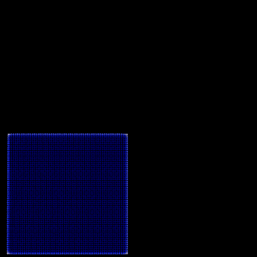
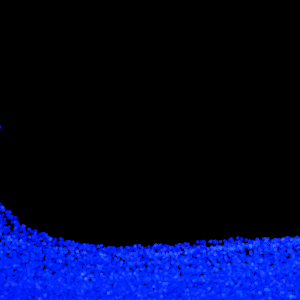
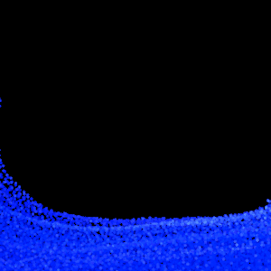
Besides, I begin to grasp the importance of the initial conditions and more particularly the initial distance between the particles. Contrary to the boids model in which initial arrangement has little impact on the simulation, PBF model are strongly dependent on the initial setup because of the density constraint. Consequently, I move away from the boids workflow where users can change the number of particles interactively and implement a set of three different scenarios (dam-break, bomb and drop). For each scenario I manually decide the number of particles and position them in a physically possible formation in order to help the simulation taking a realistic path. We can see the effect of the initial inter-particle distance on the simulation with the two following examples, the only difference between them is the size of the initial particle domain.

Large initial inter-particle distance	Small initial inter-particle distance

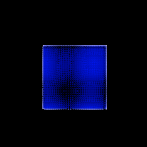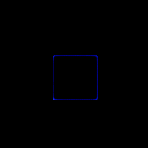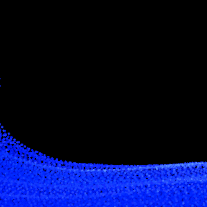
Finally, I need to improve the boundary conditions to have the standard implementation being fully functional. This is a complex subject for this type of simulation as it is hard to enforce boundary conditions on a set of moving particles. Furthermore, our constraint system is based on enforcing a similar density to every particles but how can you reach this same density value if you are against a wall and missing half your neighors and their needed contributions? Worse yet, the system locally oscillates between high and low density while trying to handle this issue, making it unstable. There is a vast literature on the subject where people use ghost particles, wall functions and other tricks at the boundaries. At first, I start by clamping particles positions within the domain but it doesn’t solve the density problem. Surprisingly, adding wall functions inspired by this implementation and this article doesn’t help much, I still see the artifacts. However, apparently favored by the ancient programming gods, I notice that the biggest unstabilities disappear while clamping the corrected positions slightly inside the domain and not at its exact borders. Don’t ask me why this trick works because I don’t have a clue yet, I will probably come back to this issue later but it gives nice visuals so far so I will stick with it for now.

Without inner domain clamping	With inner domain clamping

Advanced features

Once the basic implementation functions properly, we can add all the niceties to improve its overal behavior and the visuals. Yet, these additional features can greatly affect the performance so their usage is an esthetic-performance trade-off and we should not overdo it.

• Constraint force mixing (CFM) - It is used to prevent division by zero when computing density constraint. A must-have, it costs virtually nothing in term of computation and add some stability to the simulation.

• Artificial pressure - Adding this term is more involved in term of implementation and performance. It requires additional computation in the position correction kernel which can noticably impact framerate. However, the visual improvements are impressive and worth it in my opinion. By encouraging the particles to stay into a single pack, it generates a compelling surface tension effect.

Basic mode	BM + Artificial Pressure

• Vorticity confinement and XPSH viscosity - The most costly and difficult feature to implement. In their article, Macklin and Muller propose to compute each particle vorticity and use it to compute the vorticity confinement at every frame. We can then integrate and add this term to the particle velocity. It will increase velocity field where vorticity is present, adding some energy to active fluid area. Finally, we need to smooth the velocity field by applying the XSPH viscosity correction to balance the added vorticity energy. The whole process requires three different neighbors search and three new kernels, making it very costly. For my biggest 3D scenario, a dam-break with 130k particles, the slowdown is strong enough to be annoying but for 2D cases it brings interesting effects for an acceptable performance cost.

Basic mode (30fps)	BM + Artificial Pressure (20fps)	BM + AP + Vorticity + XSPH (16-18fps)

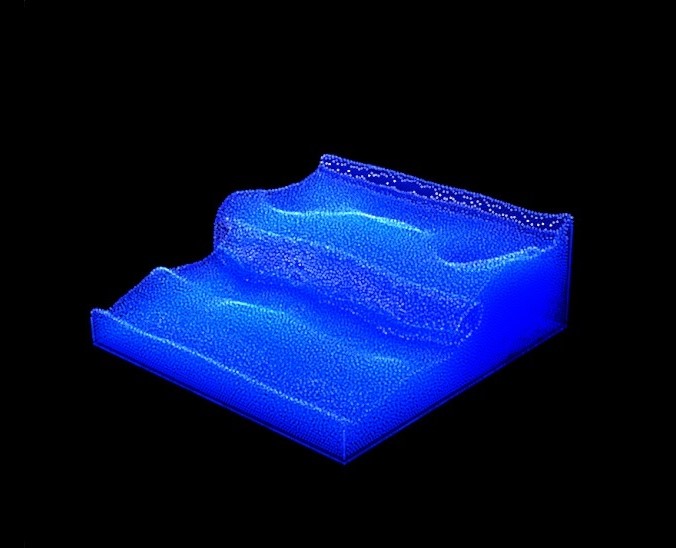
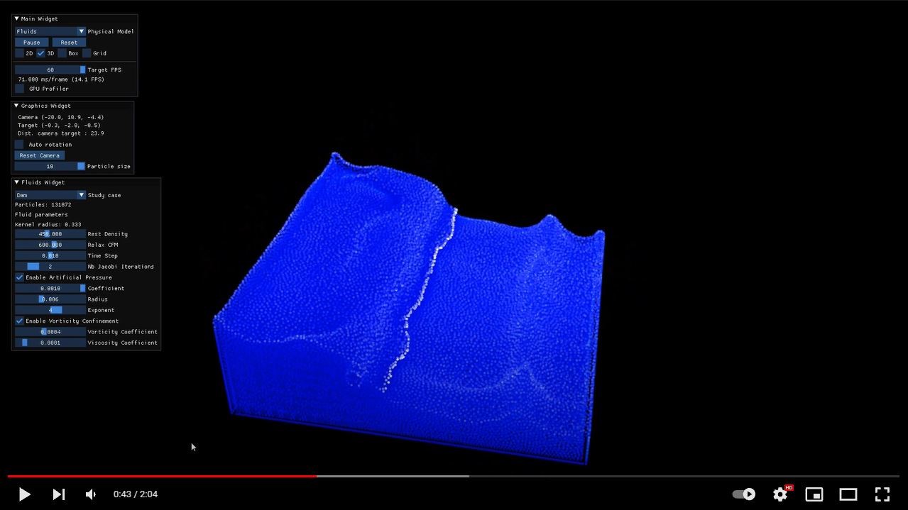
I added below the final rendering for the classical 3D dam-break scenario. Sorry for the low quality gif, it was too heavy in standard resolution. The 130k particles are processed in real-time and the model uses all the available advanced features. Notice the boundary artifacts including an unexpected high amplitude structure in the back when the main wave breaks off at the end. I will look at those boundary particles at some point but I am already very pleased with the overall result.

 

3D dam-break scenario 130k - BM + AP + Vorticity + XSPH (16 - 20 fps)

Conclusion

Finally, this long-awaited project is coming to an end! I am really happy to have successfully implemented this exciting Position Based Fluids model. The idea of implementing a fluid simulation has been stuck in my mind since I finished my master thesis, more than 5 years ago! All in all, it took me about 4 weeks, reading papers, implementing the model and debugging my way out. During this journey, I also took some time to make sure everything was coherent and the boids model still functional despite the tons of changes. In the end, I spent the last couple of days on cleaning the codebase, automating the installer packaging with CPack (RealTimeParticle 1.0 installer for Windows x64) and voila!

As always, there is still a lot of work in the backlog. I could spend more time on the rendering process to implement proper free fluid surfaces and nice lighting effects. The boundary conditions could also benefit from an upgrade. Nevertheless, I am happy with the current state of the application and I am thinking about moving away from particles for a while to experiment with new things. I will probably dive into CUDA in the near future to have access to appropriate GPU performance tools and improve my GPGPU skills. Also, a huge thank you to Maitre-Pangolin for his thorough review and wise comments.

Thanks for reading up to this point! Feel free to contact me if you have any question.

 

Full demo on Youtube