Periodic Boundary Conditions for Position Based Dynamics
Implementation of periodic boundary conditions within a Position Based Dynamics framework. Source code available here.
- Introduction
- A bit of RealTimeParticles’ history
- Revisiting our periodic BC kernel
- Applying the BCs at the right time
- Computing velocity using position corrections
- Considering the periodic BC in the Nearest Neighbor Search algorithm
- Conclusion
Introduction
The idea for this technical blog post came from a rampant bug that required a series of fixes whose increasing complexity kept my mind occupied for weeks. At the end of this fun adventure, I decided it was worth sharing with others and took the time to write it down.
So today, we are going to dive down the rabbit hole that is boundary conditions, a delicate but necessary step in any numerical simulation. More specifically, we will focus on periodic boundary conditions and how to implement them in a position-based dynamics (PBD) framework like the RealTimeParticles solver. PBD solvers are interesting because they calculate both predicted and corrected particle positions at each time step. In this situation, where should the boundary conditions be applied?
Before jumping into it, I strongly recommend going through Part 1 and Part 2 of RealTimeParticles series. This blog post brings a lot of technical details, many of which are explained in details in these previous parts.
A bit of RealTimeParticles’ history
First implementation of the boundary conditions
Back in 2021, to initiate the work on RealTimeParticles, I implemented the boids model with a good friend of mine. To obtain a variety of relevant flocking behaviors, we ended up supporting two different types of boundary conditions (BC), wall and periodic:
| Wall Boundary (2D Boids) | Periodic Boundary (2D Boids) |
|---|---|
 |  |
Here are their implementations in OpenCL:
/*
  Update position and apply periodic boundary conditions.
*/
__kernel void bd_updatePosAndApplyPeriodicBC(//Input
                                             const __global float4 *vel,     // 0
                                             //Param
                                             const          float  timeStep, // 1
                                             //Input/output
                                                   __global float4 *pos)     // 2
{
  const float4 newPos = pos[ID] + vel[ID] * timeStep;

  float4 clampedNewPos = clamp(newPos, (float4)(-ABS_WALL_X, -ABS_WALL_Y, -ABS_WALL_Z, 0.0f),
                                       (float4)( ABS_WALL_X,  ABS_WALL_Y,  ABS_WALL_Z, 0.0f));

  if (!isequal(clampedNewPos.x, newPos.x))
  {
    clampedNewPos.x *= -1.0f;
  }
  if (!isequal(clampedNewPos.y, newPos.y))
  {
    clampedNewPos.y *= -1.0f;
  }
  if (!isequal(clampedNewPos.z, newPos.z))
  {
    clampedNewPos.z *= -1.0f;
  }

  pos[ID] = clampedNewPos;
}
OpenCL implementation of a periodic boundary condition
/*
  Update position and apply wall boundary conditions on position and velocity.
*/
__kernel void bd_updatePosAndApplyWallBC(//Input/output
                                         __global float4 *vel,     // 0
                                         //Param
                                         const    float  timeStep, // 1
                                         //Input/output
                                         __global float4 *pos)     // 2


{
  const float4 newPos = pos[ID] + vel[ID] * timeStep;

  const float4 clampedNewPos = clamp(newPos, (float4)(-ABS_WALL_X, -ABS_WALL_Y, -ABS_WALL_Z, 0.0f),
                                             (float4)( ABS_WALL_X,  ABS_WALL_Y,  ABS_WALL_Z, 0.0f));

  pos[ID] = clampedNewPos;

  // Bouncing particle will have its velocity reversed and divided by half
  if (!all(isequal(clampedNewPos.xyz, newPos.xyz)))
  {
    vel[ID] *= -0.5f;
  }
}
OpenCL implementation of a wall boundary condition
As you can see, their implementation is relatively simple and straightforward. The particle domain is a cube whose center is also the center of our coordinate system, this simplifies things. Note that the wall implementation is not a no-slip BC, we simply reverse and halve the velocity of the particles hitting the walls. For the periodic one, we clamp the position coordinates to the domain boundaries, compare them to their original values, and reset them to the opposite boundaries if the comparison returns false. Two years later, I clearly see the imperfection of these conditions (we will discuss ways to improve it soon), but despite its flaws, it worked really well with the boids.
Wall BC for Position Based Fluids
Compared to the boids model, the implementation of boundary conditions in the Position Based Fluids (PBF) framework was more complex. For each time step, each particle has both predicted and corrected positions, the latter one being iteratively updated several times. On which position buffer do you apply the boundary conditions? One of them, both of them? The original Position Based Fluids paper suggests implementing the BC in the Jacobian loop which corrects the position (“perform collision detection and response”). I followed their guidelines, and after some trial and error, my version more or less worked with wall BCs by hacking some adjustments I am definitely not proud of.
/*
  Apply Bouncing wall boundary conditions on corrected position
*/
__kernel void fld_applyBoundaryCondition(__global float4 *correctedPos)
{
  correctedPos[ID] = clamp(correctedPos[ID], (float4)(-ABS_WALL_X + 0.01f, -ABS_WALL_Y + 0.01f, -ABS_WALL_Z + 0.01f, 0.0f)
                                 , (float4)(ABS_WALL_X - 0.1f, ABS_WALL_Y - 0.1f, ABS_WALL_Z - 0.1f, 0.0f)); //WIP, 0.1 and 0.01 are heuristic values to deal with boundary conditions
}
Hacked wall BCs for fluids - nothing can be better than random arbitrary numbers in the middle of your code…
Now that I see this, I wonder why I did not set the normal velocity component to zero in order to have a no-slip BC… Anyway, at that time, as I was playing with fluids, I was not interested in periodic BCs so I only implemented the wall BC and it worked relatively well despite its flaws.
What about periodic BC with Position Based Dynamics?
Suppose that despite a very typical modern life with its endless distractions, I managed to dedicate enough time to work on a new Position Based solver (new article on the subject soon). Also, assume that this solver needs periodic conditions. How should I implement it? Of course, at first I genuinely thought about simply adding the existing periodic BC to my new PBD solver, in a similar way as the current wall BC in PBF. Did it work? Not really…
 Broken periodic boundaries on vertical walls (2D PBF)
Well, it’s time to take a step back and think a little deeper…
Revisiting our periodic BC kernel
If we go back to the perodic BC OpenCL kernel presented above, one obvious flaw is the use of the OpenCL-specific function isEqual(). It looks fancy and can be vectorized, but behind the scene this is just a basic equality operator == according to the OpenCL documentation.
if (!isequal(clampedNewPos.x, newPos.x))
{
  clampedNewPos.x *= -1.0f;
}
Initial comparison within the periodic BC kernel
Float comparison is a complex topic, but long story short: using the equality operator with floats is never a good idea because it will probably return erroneous results due to their inherent limited precision and rounding. Doing this check about 60 times per second probably saves me here, in most cases at least one check will be right. An simple solution is to use the comparison operator > to compare the absolute coordinates to the domain boundaries. We could also improve this comparison by adding some tolerance and checking the absolute margin between the particle and the boundary, or even take it further and focus on the relative margin but I think this is sufficient for now.
if (fabs(newPos.x) > ABS_WALL_X)
New comparison, switching from the == operator to the > one
Another thing that annoys me is the fact that even if we correctly detect a particle that must be transferred to the opposite boundary, we don’t take into account the actual distance traveled by the particle once it has crossed the initial wall before applying the BC.
pos[ID] = clampedNewPos;
Initial implementation simply resetting the position to the opposite boundary
That’s a bit clumsy, fortunately we can solve this pretty easily by simply keeping the distance traveled through the boundary.
pos[ID].x = newPos.x - 2 * clampedNewPos.x; // delta.x = newPos.x - clampedNewPos.x directly incorporated here
New implementation taking into account the distance traveled through the boundary
 Red particle crosses periodic boundary while preserving its motion
Here is the final boundary conditions kernel where we apply a mix of periodic and wall BCs. Note the absence of a no-slip condition for the wall, this is not necessary in this position based framework, because the velocity is calculated right after as the difference between the predicted and corrected position.
/*
  Apply periodic boundary conditions for xz directions
  Apply wall boundary conditions for y direction
*/
__kernel void cld_applyMixedBoundaryConditions(//Input/output
                                               __global float4 *predPos) // 0
{
  const float4 newPos = predPos[ID];


  const float4 clampedNewPos = clamp(newPos, (float4)(-ABS_WALL_X, -ABS_WALL_Y, -ABS_WALL_Z, 0.0f),
                                             (float4)( ABS_WALL_X,  ABS_WALL_Y,  ABS_WALL_Z, 0.0f));

  if (fabs(newPos.x) > ABS_WALL_X)
  {
    predPos[ID].x = newPos.x - 2 * clampedNewPos.x; // periodic BC, keeping delta.x
  }
  if (fabs(newPos.y) > ABS_WALL_Y)
  {
    predPos[ID].y = clampedNewPos.y; // wall BC
  }
  if (fabs(newPos.z) > ABS_WALL_Z)
  {
    predPos[ID].z = newPos.z - 2 * clampedNewPos.z; // periodic BC, keeping delta.z
  }
}
Final mixed BCs with vertical periodic boundaries preserving particles motions
Does it solve my initial problem? Not at all, let’s jump to the next fix.
Applying the BCs at the right time
The PBF article describes in detail the position-based algorithm and its main Jacobian correction loop, but it doesn’t say much about how to add the BCs to the mix or even a spatial partitioning framework essential to obtain decent performance. This is understandable because its goal is to describe a new way of simulating fluids, not to discuss any secondary algorithm implementation. However due to their absence in the paper, we can easily forget about the relation between spatial partitioning and BCs. Basic spatial partitioning involves dividing the particle domain into cells, identifying which cell contains which particle, and grouping neighboring particles based on the cell they belong to (see Part 1). With periodic boundaries, a particle might well end up in a different cell with completely different neighbors if it crosses a boundary. So we really need to apply BCs before doing any spatial partitioning. Otherwise the Nearest Neighbors Search (NNS) based on it might be incorrect near the boundaries.
In a simplified pseudo code, the ideal implementation for a given time step would then be:
PredictPosition();

// Jacobian loop, correcting positions to fit constraints
for (int iter = 0; iter < m_nbJacobiIters; ++iter)
{
  ApplyBCs();
  CreateSpatialPartitioning();
  ComputeCorrectionUsingNeighbors();
  CorrectPosition();
}

UpdateVelocity();
Ideal PBF implementation with spatial partitioning done once per position correction
In my PBF implementation, as spatial partitioning and associated buffer sorting were relatively expensive, I made the decision to take them out of the Jacobian loop. This is a risky trade-off between performance and correctness. As the partitioning is only done once per frame, we assume that during the correction the particles remain in the same cell. This only works if the particle velocity is not too high.
So the real implementation looks like this:
PredictPosition();
CreateSpatialPartioning(); // Costly operation out of the loop

// Jacobian loop, correcting positions to fit constraints
for (int iter = 0; iter < m_nbJacobiIters; ++iter)
{
  ApplyBCs();
  ComputeCorrectionUsingNeighbors();
  CorrectPosition();
}

UpdateVelocity();
Current PBF implementation (broken) with spatial partioning done once per frame
Well, this is clearly wrong. Focusing on performance, I blindly accepted the trade-off regarding potential particles changing cells during the position correction, but totally forgot about BCs. I said before that BCs should always be applied before spatial partitioning. We just don’t do it here, not even for the prediction step which is probably the most important one because that’s where the positions change the most.
For the fluid simulations where I only use wall BCs, the positions being clamped, the approximation still looks visually acceptable and I did not notice the obvious flaw. But when I start using periodic BCs, it’s a different story. Indeed, with periodic boundaries, one particle can move the size of the domain, it’s hard to have a meaningful partitioning if it doesn’t take this type of displacement into account.
So the fixed implementation looks like this:
PredictPosition();
ApplyBCs();
CreateSpatialPartioning(); // Costly operation out of the loop

// Jacobian loop, correcting positions to fit constraints
for (int iter = 0; iter < m_nbJacobiIters; ++iter)
{
  ComputeCorrectionUsingNeighbors();
  CorrectPosition();
  ApplyBCs();
}

UpdateVelocity();
Fixed PBF implementation with spatial partioning done once and correct BCs handling
Is it better? Way better. Does it fix my issue? Nope, so better keep going!
Computing velocity using position corrections
At this point, periodic BCs still don’t work in general but a global constant speed enforced on all the particles gives the right result using them. It gives me two clues, firstly, I’m not very far from the truth, secondly, the problem lies in the correction loop itself. Indeed, the particle velocity is based on the difference between the final corrected position and the position at the previous time step, if the velocity is wrong it must come from there.
/*
  Update velocity buffer
*/
__kernel void fld_updateVel(//Input
                            const __global float4 *newPos,    // 0
                            const __global float4 *prevPos,   // 1
                            //Param
                            const     FluidParams fluid,      // 2
                            //Output
                                  __global float4 *vel)       // 3
{
  // Clamping velocity and preventing division by 0
  vel[ID] = clamp((newPos[ID] - prevPos[ID]) / (fluid.timeStep + FLOAT_EPS), -MAX_VEL, MAX_VEL);
}
OpenCL kernel updating the particle velocity
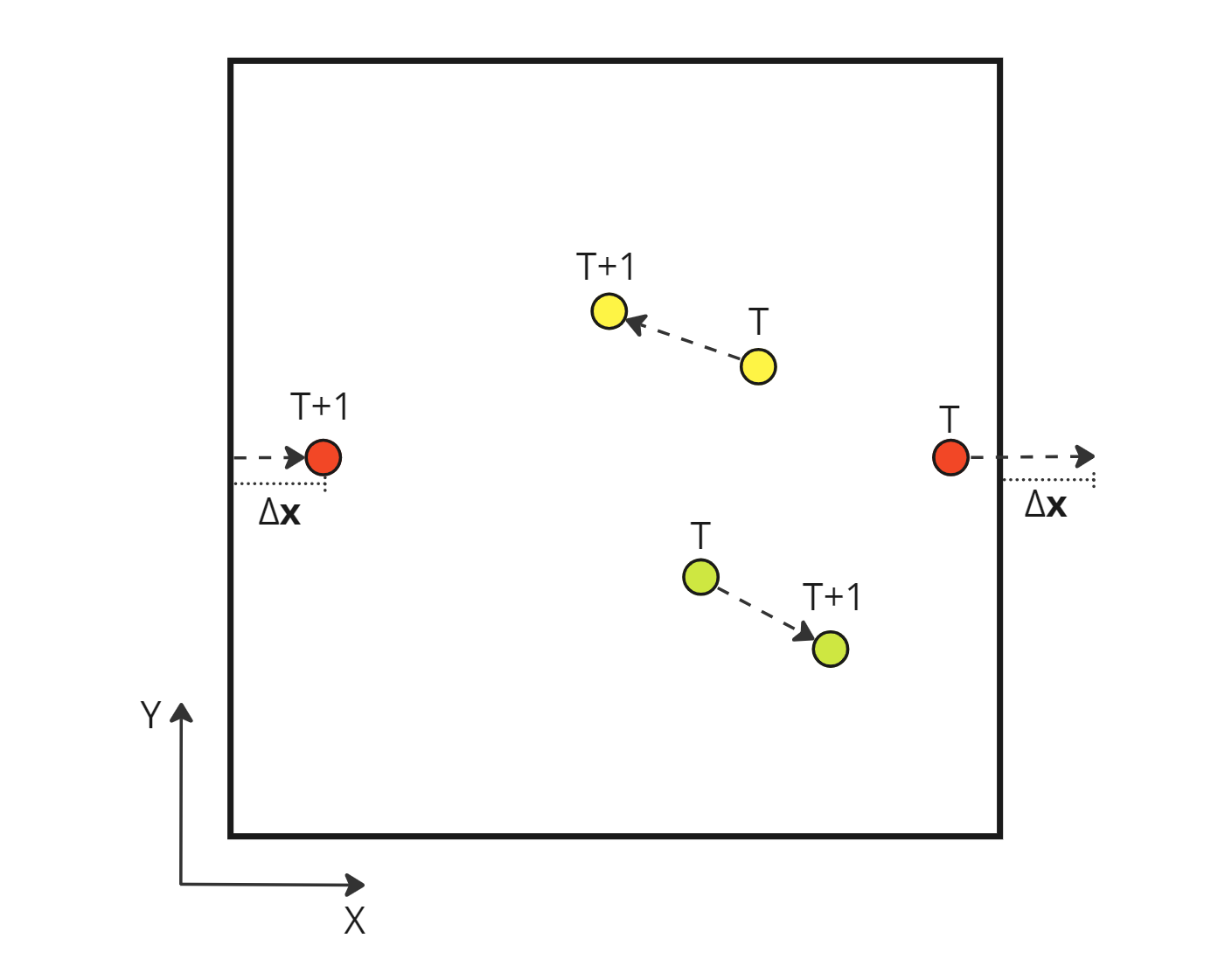
Drawing a diagram of the situation makes me realize the issue. If a particle crosses a periodic boundary, its new position differs greatly from the previous one due to the particle’s jump to the opposite boundary. Therefore, the computed velocity is suddenly huge for that time step. This explains the exponential increase in the velocity for some particles in the initial erroneous behavior.
 Absolute displacement of a particle during a time step
If we use this absolute displacement, we end up with an incorrect velocity which omits any boundary crossing: \[\begin{aligned} \mathbf{v} = \frac{\Delta \mathbf{x}}{\Delta T} = \frac{ \mathbf{x}_{T+1} - \mathbf{x}_T }{ (T+1) - T} \\ \end{aligned}\]
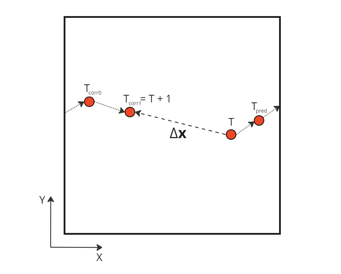
One way to solve this problem is to consider the sum of corrections applied on the initial position, not the absolute distance between this initial position and the final corrected one. Indeed, this absolute distance can contain jumps between periodic boundaries, in other words erroneous distances not traveled by the particles. We can obtain the actual distance traveled by the particle by creating a new buffer totalCorrection which will contain all the increment adjustments made to the initial position, i.e. the initial prediction and all the subsequent corrections. The velocity is then calculated using this new buffer.
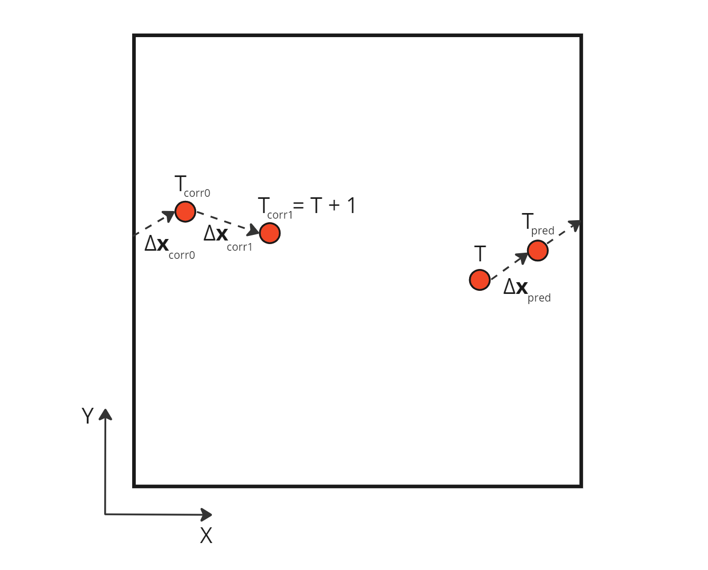 Sum of the relative corrections applied during a time step
Using those relative corrections, we can compute the correct velocity which takes into account the boundary crossing: \[\begin{aligned} \mathbf{v} = \frac{\Delta \mathbf{x}_{pred} + \sum \Delta \mathbf{x}_{corr \space i}}{\Delta T} = \frac{ \Delta \mathbf{x}_{pred} + \Delta \mathbf{x}_{corr \space 0} + \Delta \mathbf{x}_{corr \space 1} }{ (T+1) - T} \\ \end{aligned}\]
Here is the implementation of the new workflow in OpenCL:
/*
  Predict fluid particle position and update velocity by integrating external forces
*/
__kernel void cld_predictPosition(//Input
                                  const __global float4 *pos,        // 0
                                  const __global float4 *vel,        // 1
                                  const __global float  *buoyancy,   // 2
                                  //Param
                                  const     CloudParams cloud,       // 3
                                  //Output
                                        __global float4 *predPos,     // 4
                                        __global float4 *totCorrPos)    // 5
{
  // No need to update global vel, as it will be reset later on
  const float4 predVel = vel[ID] + (float4)(0.0f, buoyancy[ID], 0.0f, 0.0f) * cloud.timeStep;
  // Init totCorrPos with prediction dist
  totCorrPos[ID] = predVel * cloud.timeStep;


  predPos[ID] = pos[ID] + predVel * cloud.timeStep;
}

/*
  Sum correction positions
*/
__kernel void fld_updateTotCorrPosition(//Input
                                  const __global float4 *corrPos, // 0
                                  //Output
                                        __global float4 *totCorrPos) // 1
{
  totCorrPos[ID] += corrPos[ID];
}


/*
  Update velocity buffer
*/
__kernel void fld_updateVel(//Input
                            const __global float4 *totCorrPos, // 0
                            //Param
                            const     FluidParams fluid,       // 1
                            //Output
                                  __global float4 *vel)        // 2
{
  // Clamping velocity and preventing division by 0
  vel[ID] = clamp((totCorrPos[ID]) / (fluid.timeStep + FLOAT_EPS), -MAX_VEL, MAX_VEL);
}
OpenCL kernels computing totalCorrection buffer then using it for velocity
Finally, the visual result is much better! There are no more blinking particles, the periodic BCs no longer act as time warp portals with the particles. However they still have some visible effect on the particles, a perfect periodic BC should not affect the particles traversing it. No time to rest, the investigation is not over!
Straining effect, note the left particles struggling to enter the domain
Considering the periodic BC in the Nearest Neighbor Search algorithm
There is a clear loss of cohesion in the stock of particles crossing the periodic boundary, as if the BC was acting as a sieve. The particles seem reluctant to cross the boundary. For what? They generally won’t go somewhere if it means reducing their density, i.e. losing some connections with neighbors. But in crossing this periodic boundary, they should not lose any, as their neighbors are still right behind, close to them and ready to follow them. Oh, it finally hits me. The Nearest Neighbor Search (NNS) algorithm does not take into account periodic neighbor cells: neighbor particles on the other side of a periodic boundary are omitted in all calculations. In other words, currently for a particle, crossing the boundary means suddenly losing all its previous neighbors, impacting the efforts applied to it and therefore its movement.
 NNS correctly taking into account periodic neighbor cells
This is a serious flaw in my NNS algorithm implementation. I should have seen it sooner but I probably pushed the problem to the back of my mind because it seemed difficult to implement. Literature talks about ghost particles with fake density or even duplication of boundary neighbor particles, but I really didn’t like that. It means potential dynamic buffers and higher memory consumption. I think I have a better idea that should match my simple case. With my box domain, I know the grid resolution and I know the index of my current cell, using this information I can surely calculate the index of its direct periodic neighboring cells, if any. Properly fetching periodic neighbor cells should solve my NNS problem.
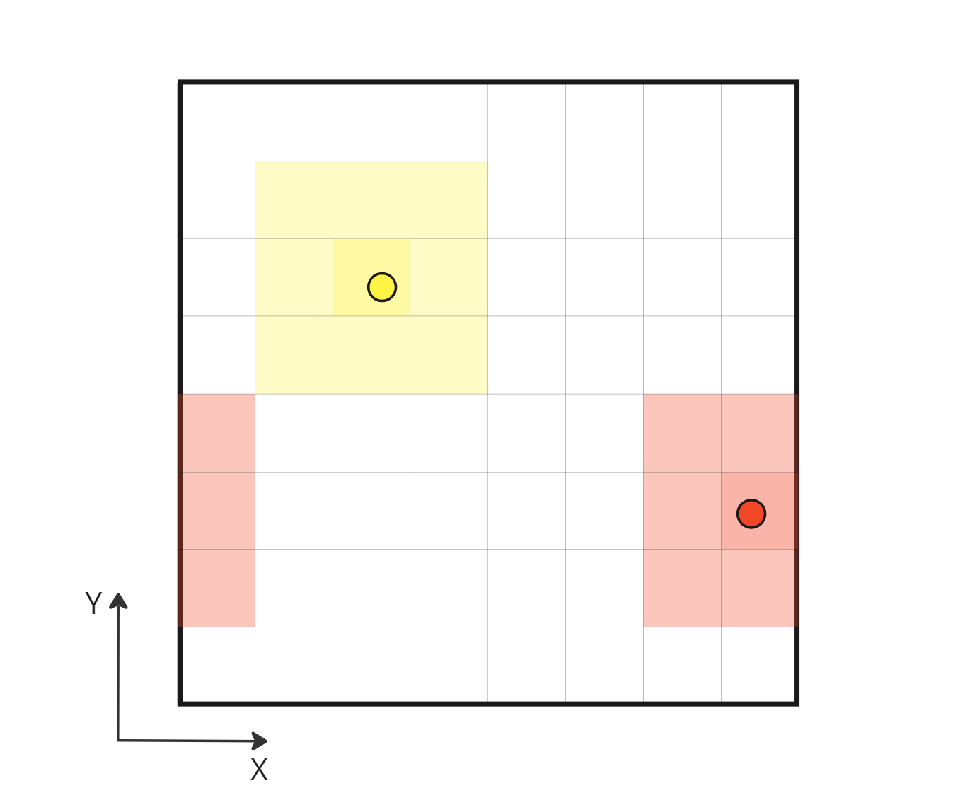
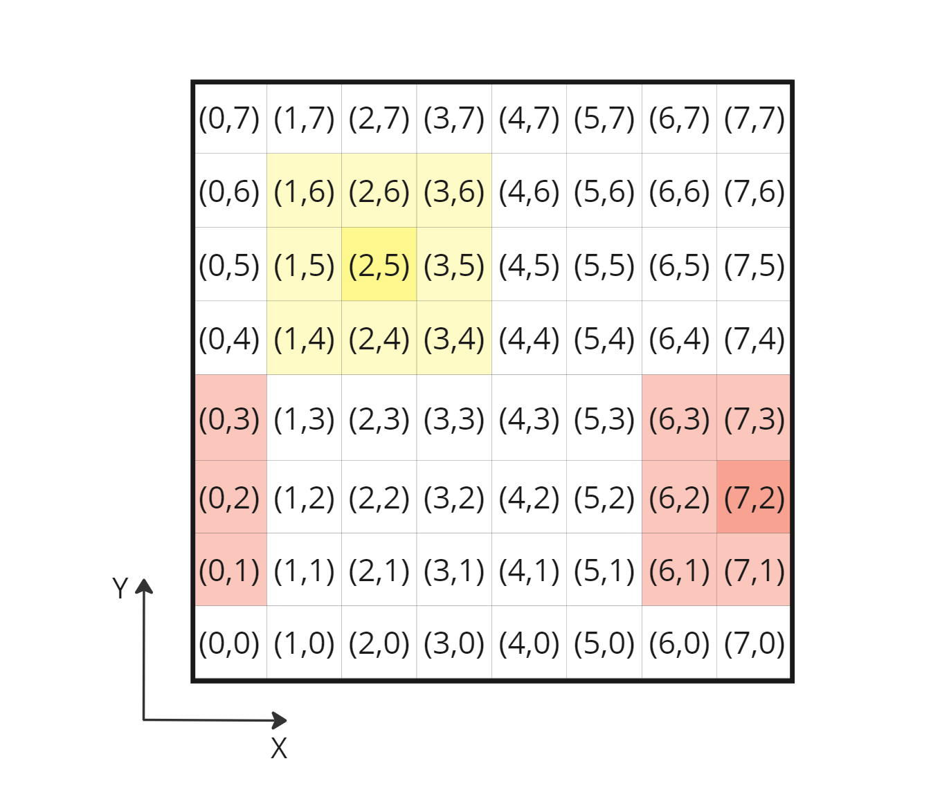 Spatial partitioning and cell indices in 2D, computing periodic neighbor indices using particle cell index is straightforward
After experimenting on paper, I end up with this formula:
// Initial formula to obtain a neighbor cell index in 3D
// cellNIndex3D = convert_int3(currCellIndex3D) + (int3)(iX, iY, iZ);

// New formula taking into account periodic neighbor cells
cellNIndex3D = (convert_int3(currCellIndex3D) + (int3)(iX, iY, iZ) + gridResXYZ) % gridResXYZ;
Corrected 3D cell index formula retrieving periodic neighbor cell indices
It’s nice on paper but unfortunately it doesn’t help anything and this lack of improvement is driving me crazy. It’s 2am when I finally implement it and I really thought ths would solve my problem. But then it hits me again! This is the right fix but I need to go down another layer, indeed the SPH kernels Part 1 have no effect beyond their limited radius. When we consider the absolute distance between a selected particle and its periodic neighbors, this distance is always larger than the SPH effect radius and therefore the periodic neighbors contribution is zero.
In other words, we are correctly retrieving all the neighbor particles (periodic or not) thanks to the initial fix, but all periodic ones don’t have any effect on the selected particle for now. Let’s adjust it so the periodic neighbors have a real contribution during the NNS:
// 27 cells to visit, current one + 3D neighbors
for (int iX = -1; iX <= 1; ++iX)
{
 for (int iY = -1; iY <= 1; ++iY)
 {
   for (int iZ = -1; iZ <= 1; ++iZ)
   {
     signAbsWall = (float4)(0.0f);

     // Computing 3D index of the current neighbor cell
     cellNIndex3D = (cellIndex3D + (int3)(iX, iY, iZ) + gridResXYZ) % gridResXYZ;

     // Periodic BC for x, periodic neighbors must be considered
     if((cellIndex3D.x + iX) >= GRID_RES_X) signAbsWall.x = 2.0f;
     else if((cellIndex3D.x + iX) < 0) signAbsWall.x = -2.0f;

     // Wall BC for y, out of domain cells are discarded
     if(((cellIndex3D.y + iY) >= GRID_RES_Y) || ((cellIndex3D.y + iY) < 0)) continue;

     // Periodic BC for z, periodic neighbors must be considered
     if((cellIndex3D.z + iZ) >= GRID_RES_Z) signAbsWall.z = 2.0f;
     else if((cellIndex3D.z + iZ) < 0) signAbsWall.z = -2.0f;

     // Computing 1D index of the current neighbor cell
     cellNIndex1D = (cellNIndex3D.x * GRID_RES_Y + cellNIndex3D.y) * GRID_RES_Z + cellNIndex3D.z;

     // Retrieving indices of all the particles in this cell
     startEndN = startEndCell[cellNIndex1D];

     for (uint e = startEndN.x; e <= startEndN.y; ++e)
     {
       fluidDensity += poly6(pos - predPos[e] - absWallXYZ * signAbsWall, EFFECT_RADIUS); // poly6 is the SPH kernel used to compute density
     }
   }
 }
}
Adjusted SPH kernel with correct NNS
The periodic BC is hardcoded in the NNS algorithm for X and Z direction, this is not perfect but this will do for now. Notice how we adjust the distance between particles sent to the SPH kernel, so that the periodic neighbors contribute to the particle density.
 Periodic boundary fully functioning in 2D
Does it work? Yes! The particles are finally crossing the periodic boundaries without any visible change in behavior.
Conclusion
What a journey. It took a long time but we got there. If you are still here, thanks you so much for following me this far. I hope that it will be helpful at least for the few tormented souls who are also looking at implementing similar periodic boundary conditions within a Position Based Dynamics framework.
To summarize, over the course of this blog post, I went through a series of fixes and adjustments of progressive complexity in order to enable periodic boundary conditions in my Position Based Dynamics framework. The challenge came in part from the spatial partitioning implemented to accelerate our Nearest Neighbor Search (NNS) algorithm.
Properly implementing this boundary condition was tricky, but it was a necessary first step towards integrating my future solver. This one will be the main subject of my next article, stay tuned!
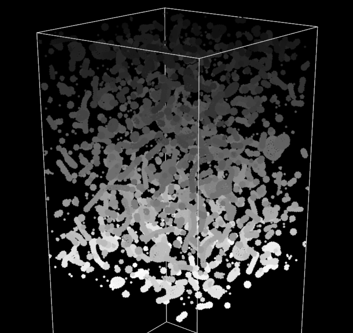
 Periodic boundary 3D with a new PBD model in preparation